Designing and Training a Neural Network in Python

In this article, we will implement the sentiment analysis neural network described in What is a neural network?. For a thorough explanation of how neural networks work, refer to that post. Here, we focus on the practical implementation of that example in Python.

All the code and resources for this tutorial are available in the AssistiveComputing-Tutorials GitHub repository. Feel free to clone or fork the repository to follow along or experiment with the code.

Background

Let’s review the example neural network that analyzes a movie review to determine whether it is positive or negative. Our network will use six input features:

1. Word Count
2. Average Word Length
3. Number of Positive Words
4. Number of Negative Words
5. Contains “excellent” (1 if yes, 0 if no)
6. Contains “terrible” (1 if yes, 0 if no)

The network structure described in the article has the following structure:

• Input Layer: 6 nodes (one for each feature)
• Hidden Layer 1: 10 nodes
• Hidden Layer 2: 5 nodes
• Output Layer: 1 node (to predict sentiment: 1 for positive, 0 for negative)

Step 1: Setting Up the Environment

We will use the following libraries in this tutorial:

1. pandas: We use pandas to load our CSV file into a DataFrame and to select specific columns for our features and target variable.

   df = pd.read_csv('synthetic_movie_reviews.csv')
   X = df[['Word Count', 'Average Word Length', 'Positive Words', 'Negative Words', "Contains 'excellent'", "Contains 'terrible'"]]
   y = df['Positive Words'] > df['Negative Words']
   

2. numpy: We use numpy in our data generation script to calculate the average word length.

   avg_word_length = np.mean([len(word) for word in review_words])
   

3. scikit-learn: We use scikit-learn for two main purposes:

   a. Splitting our data into training and test sets:

   from sklearn.model_selection import train_test_split
   X_train, X_test, y_train, y_test = train_test_split(X, y, test_size=0.2, random_state=42)
   

   b. Standardizing our features:

   from sklearn.preprocessing import StandardScaler
   scaler = StandardScaler()
   X_train_scaled = scaler.fit_transform(X_train)
   X_test_scaled = scaler.transform(X_test)
   

4. TensorFlow: We use TensorFlow (specifically, the Keras API) to build, compile, and train our neural network:

   from tensorflow.keras.models import Sequential
   from tensorflow.keras.layers import Dense
   
   model = Sequential([
       Dense(10, activation='relu', input_shape=(X_train.shape[1],)),
       Dense(5, activation='relu'),
       Dense(1, activation='sigmoid')
   ])
   
   model.compile(optimizer='adam', loss='binary_crossentropy', metrics=['accuracy'])
   
   history = model.fit(X_train_scaled, y_train, epochs=50, batch_size=32, validation_split=0.2, verbose=1)
   

5. matplotlib: We use matplotlib to create visualizations of the model’s training process, allowing us to see how accuracy changes over time.

We import the libraries with the following code:

import pandas as pd
import numpy as np
from sklearn.model_selection import train_test_split
from sklearn.preprocessing import StandardScaler
import tensorflow as tf
from tensorflow.keras.models import Sequential
from tensorflow.keras.layers import Dense
import matplotlib.pyplot as plt

You can install the necessary libraries using pip:

pip install pandas numpy scikit-learn tensorflow matplotlib

Step 2: Generating Synthetic Data

For this tutorial, we use synthetic data to train our model. Synthetic data is an inexpensive source of data for training since it is generated automatically. It also avoids privacy issues that may way arise with real data. Using synthetic data can be convenient for testing a design but it lacks the quality of real data. Here is the code to generate the data for this tutorial:

import random
import numpy as np
import pandas as pd

positive_words = ["good", "great", "fantastic", "amazing", "excellent", "wonderful", "positive", "enjoyable", "pleasant", "satisfying"]
negative_words = ["bad", "terrible", "awful", "horrible", "negative", "poor", "disappointing", "unpleasant", "dismal", "unsatisfactory"]

def generate_review():
    word_count = random.randint(50, 200)
    review_words = []
    positive_word_count = 0
    negative_word_count = 0
    contains_excellent = 0
    contains_terrible = 0

    for _ in range(word_count):
        if random.random() > 0.5:
            word = random.choice(positive_words)
            positive_word_count += 1
            if word == "excellent":
                contains_excellent = 1
        else:
            word = random.choice(negative_words)
            negative_word_count += 1
            if word == "terrible":
                contains_terrible = 1
        review_words.append(word)

    review_text = " ".join(review_words)
    avg_word_length = np.mean([len(word) for word in review_words])
    positive_review = 1 if positive_word_count > negative_word_count else 0

    return {
        "Review Text": review_text,
        "Word Count": word_count,
        "Average Word Length": avg_word_length,
        "Positive Words": positive_word_count,
        "Negative Words": negative_word_count,
        "Contains 'excellent'": contains_excellent,
        "Contains 'terrible'": contains_terrible,
        "Positive Review": positive_review
    }

# Generate dataset
number_reviews = 5000
reviews = [generate_review() for _ in range(number_reviews)]
df = pd.DataFrame(reviews)

# Save to CSV
df.to_csv('synthetic_movie_reviews.csv', index=False)

This code creates a dataset of 5000 synthetic movie reviews, each with the features we need for our neural network.

Step 3: Preparing the Data

Now that we have the data, We need to prepare it for training. Preparing the data involves the following steps:

1. Load the synthetic data
2. Select the features (X) and target variable (y)
3. Split the data into training and testing sets
4. Standardize the features to have mean 0 and standard deviation 1

Here is the code for these steps:

# Load the synthetic dataset
df = pd.read_csv('synthetic_movie_reviews.csv')

# Features and target variable
X = df[['Word Count', 'Average Word Length', 'Positive Words', 'Negative Words', "Contains 'excellent'", "Contains 'terrible'"]]
y = df['Positive Words'] > df['Negative Words']  # Target: more positive words than negative

# Convert boolean target to int
y = y.astype(int)

# Split the data into training and testing sets
X_train, X_test, y_train, y_test = train_test_split(X, y, test_size=0.2, random_state=42)

# Standardize the features
scaler = StandardScaler()
X_train_scaled = scaler.fit_transform(X_train)
X_test_scaled = scaler.transform(X_test)

Step 4: Building the Neural Network

We use TensorFlow to construct the neural network:

# Define the neural network model
model = Sequential([
    Dense(10, activation='relu', input_shape=(X_train.shape[1],)),
    Dense(5, activation='relu'),
    Dense(1, activation='sigmoid')  # Output layer for binary classification
])

# Compile the model
model.compile(optimizer='adam', loss='binary_crossentropy', metrics=['accuracy'])

This code creates a Sequential model (i.e., a simple feedforward neural network) with the structure we described in the article:

• Input layer: Implicitly defined by the input_shape
• First hidden layer: 10 nodes with ReLU activation
• Second hidden layer: 5 nodes with ReLU activation
• Output layer: 1 node with sigmoid activation (for binary classification)

Step 5: Training the Model

Now we have a network with the desired structure that is ready for training:

# Train the model
history = model.fit(X_train_scaled, y_train, epochs=50, batch_size=32, validation_split=0.2, verbose=1)

This code will train the model for 50 epochs, using batches of 32 samples. The validation_split=0.2 parameter sets aside 20% of the training data for validation.

If a model’s performance on the training data improves while its performance on the validation data stagnates or worsens, then the model may be overfitting. If a model performs well on both training and validation data, then it suggests that the model has learned general patterns rather than specific examples.

Step 6: Visualizing the Training Process

By visualizing the training process can monitor how the model is learning. Let’s create a plot for the training and validation accuracy:

import matplotlib.pyplot as plt

# Plot training & validation accuracy
plt.figure(figsize=(10,6))
plt.plot(history.history['accuracy'])
plt.plot(history.history['val_accuracy'])
plt.title('Model Accuracy')
plt.ylabel('Accuracy')
plt.xlabel('Epoch')
plt.legend(['Train', 'Validation'], loc='upper left')
plt.show()

This code creates a plot that shows how the accuracy improves for both training and validation sets over epochs. The resulting plot might look similar to Figure 1.

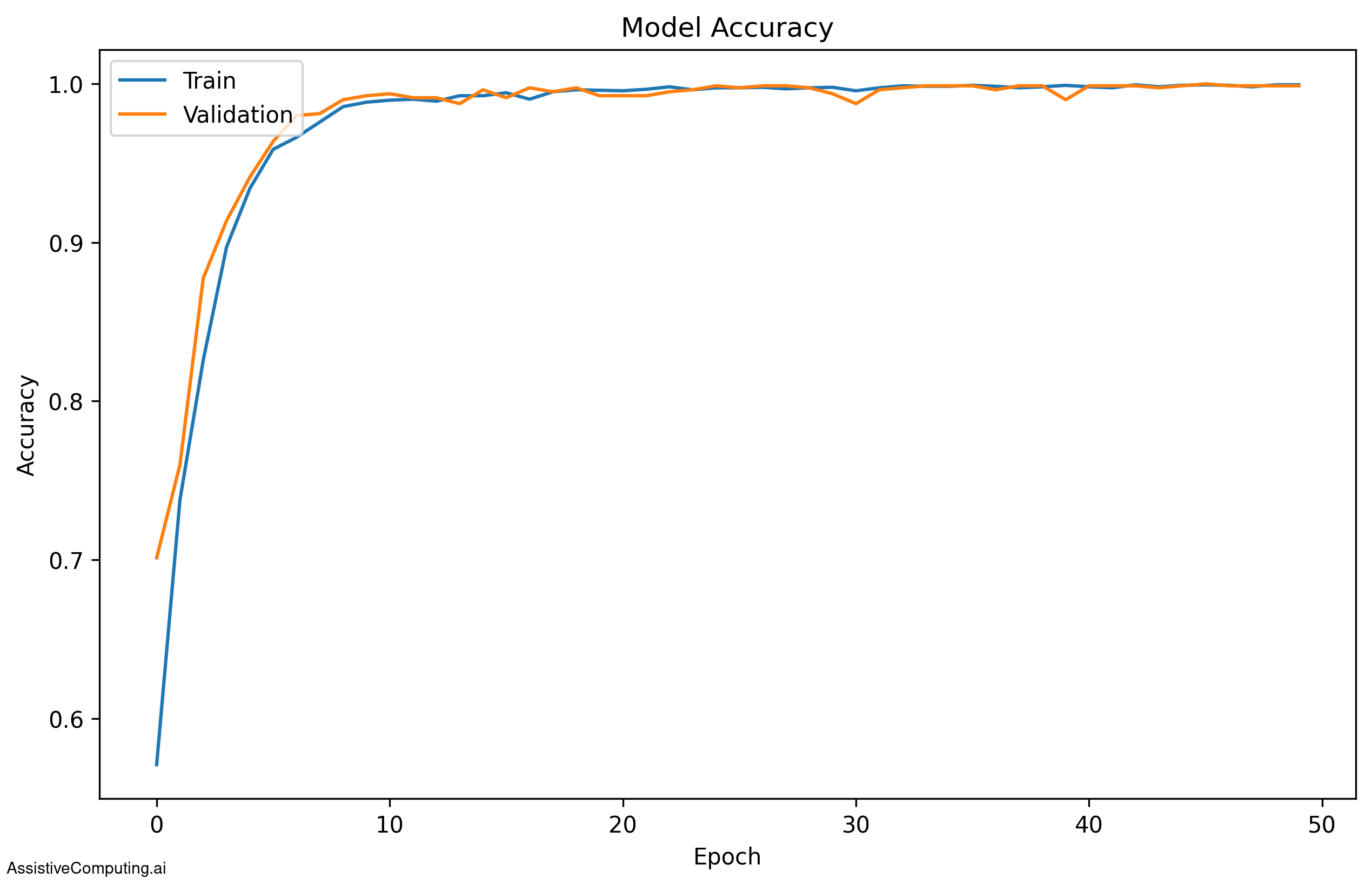Figure 1: Model accuracy over training epochs for both training and validation sets

What to look for in this plot:

1. Both training and validation accuracy should increase (generally) over time.
2. If the training accuracy is much higher than the validation accuracy, especially in later epochs, then the model may be overfitting.
3. If both accuracies are low and not improving much, then the model might be underfitting.

Step 7: Evaluating the Model

Finally, let’s evaluate our model on the test set:

# Evaluate the model
loss, accuracy = model.evaluate(X_test_scaled, y_test)
print(f'Test Accuracy: {accuracy:.2f}')

This will compute the accuracy of our model on data it has not seen yet. The accuracy tells us the proportion of reviews that are classified correctly.

Conclusion

Congratulations! You have implemented and trained a neural network for sentiment analysis. This tutorial guided you through the process of:

1. Generating synthetic data
2. Preparing the data for training
3. Building a neural network with the structure described in our article
4. Training the network
5. Evaluating its performance

This is a simplified example using synthetic data. Real-world sentiment analysis often involves more complex techniques, especially in processing text data. However, this tutorial provides a foundation for understanding how to implement a basic neural network for classification tasks.

Feel free to experiment with the network structure. You can try different hyperparameters or even use real movie review data to see how the performance changes.